Background and Strategy
This task covers the creation of those Local Transform objects previously identified as necessary to deliver data into the Natural object layer.
As with the prior task, it is difficult to give specific advice for development work that is so inherently variable. However, the best practice guidance on the following typical subtasks may be helpful:
1. Setting the object and table names.
Teams will likely want to establish object and table naming conventions. Because in most cases there is a direct, one-to-one relationship between a Local Transform object and its terminal Natural object, the recommended convention is to base the former's object and table names on the latter, along with an identifier for the source sytem to avoid naming collisions with Local Transform objects from other sources building toward the same Natural object.
For example, the DataCo organization's Local Transform object for source system DS for terminal Natural object Patients (table name ursa.no_ursa_core_pat_001) might be named "Source DS Patients LT" (with table name ursa.lt_dataco_ds_ursa_core_pat_001).
2. Selecting the appropriate object type.
For data that must be conformed to a timeline structure, using a Simple Timeline or Complex Timeline is typically necessary to ensure non-overlappingness of timeline periods.
Simple Timelines resolve overlapping periods by truncating earlier period end dates to end the period when the next period starts; for example, the overlapping periods in the following source data:
| Patient ID | Period Start Date | Period End Date | Plan ID |
|---|---|---|---|
| 1 | 1/1/2022 | 10/1/2022 | P1 |
| 1 | 6/1/2022 | 1/1/2023 | P1 |
...would be resolved to the following via a Simple Timeline:
| Patient ID | Period Start Date | Period End Date | Plan ID |
|---|---|---|---|
| 1 | 1/1/2022 | 6/1/2022 | P1 |
| 1 | 6/1/2022 | 1/1/2023 | P1 |
It is recommended to use a Simple Timeline to ensure clean timeline data for Natural objects like Patient-Plan Timelines of Plan Membership.
Complex Timelines can be used to capture and integrate information from multiple timelines; for example:
| Patient ID | Period Start Date | Period End Date | Plan ID | Is Plan Coverage Type Medical | Is Plan Coverage Type Pharmacy |
|---|---|---|---|---|---|
| 1 | 1/1/2022 | 10/1/2022 | P1 | 0 | 1 |
| 1 | 6/1/2022 | 1/1/2023 | P2 | 1 | 0 |
...might be transformed into the following via a Complex Timeline:
| Patient ID | Period Start Date | Period End Date | Plan ID | Is Plan Coverage Type Medical | Is Plan Coverage Type Pharmacy |
|---|---|---|---|---|---|
| 1 | 1/1/2022 | 6/1/2022 | P1 | 0 | 1 |
| 1 | 6/1/2022 | 10/1/2022 | P2 | 1 | 1 |
| 1 | 10/1/2022 | 1/1/2023 | P2 | 1 | 0 |
Notice that all the information from the original two period is preserved, with the resulting timeline capturing the fact that during the overlapping period of enrollment in P1 and P2 the patient has both medical and pharmacy coverage.
It is recommended to use a Complex Timeline to prepare data for Natural objects like Patient-Source Timelines of Data Coverage that involve aggregating information from potentially multiple (potentially overlapping) patient-periods.
For more straightforward Local Transform objects -- those that might require a number of joins but are not related to timelines, and which don't require the union of records from more than one upstream object -- , the simple but flexible Single Stack object type is a reasonable default option.
In cases where there is a need to union records from multiple upstream sources, or where there might be a future need to do so, Integrator objects are recommended. In addition to this native handling of unioning multiple stacks, the output fields of an Integrator objects can be imported from the structure of another object (such as the terminal Natural object for that Local Transform object), which can be a convenient way to set up a Local Transform object to output all the fields needed for a downstream Natural Object.
3. Removing duplicate records.
It isn't uncommon for source data to contain exact duplicate records. For example, this can easily happen -- intentionally or not -- under a number of scenarios involving the ongoing import of multiple files from the same source system.
Note that care must be taken to discern transactional claims or billing records -- which often repeat the vast majority of field values -- from "true" duplicates in which every single field value (with the exception of metadata fields, like filename or source data effective date, etc.) is repeated in two or more records.
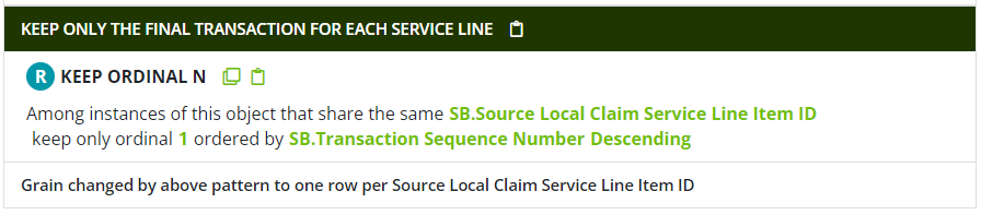
As a general rule, true duplicates should be removed in the Local Transform Layer. This can be accomplished most easily using the Keep Ordinal N pattern with the partition field(s) set to be the desired post-deduplication primary key for the record. For example, duplicate records like this:
| Source Local Transaction Header ID | Source Local Patient ID | Claim Covered Start Date | Claim Covered End Date | CMS Type of Bill Code | Claim Plan Paid Amount | Source Data Effective Datetime |
|---|---|---|---|---|---|---|
| 100 | 1 | 1/1/2022 | 1/4/2022 | 111 | 500 | 3/1/2022 |
| 100 | 1 | 1/1/2022 | 1/4/2022 | 111 | 500 | 4/1/2022 |
...could use the following configuration of Keep Ordinal N:
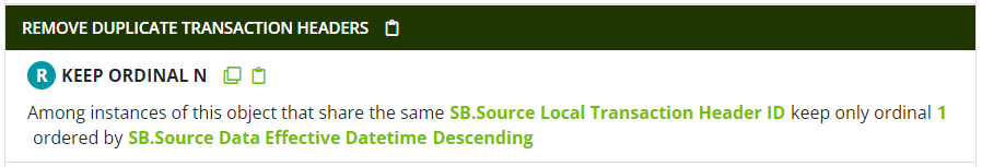
The ordering by Source Data Effective Datetime descending simply preserves the most advanced Source Data Effective Datetime value, which best reflects the freshness of that record. The resulting record is:
| Source Local Transaction Header ID | Source Local Patient ID | Claim Covered Start Date | Claim Covered End Date | CMS Type of Bill Code | Claim Plan Paid Amount | Source Data Effective Datetime |
|---|---|---|---|---|---|---|
| 100 | 1 | 1/1/2022 | 1/4/2022 | 111 | 500 | 4/1/2022 |
4. Incorporating information from other source tables
Source data are often highly normalized, meaning there may be a number of dimension or lookup tables that will need to be joined in to form a complete picture of a record. The Local Transform Layer is the appropriate place to perform these joins.
All source tables involved in this exercise should have already passed through the Semantic Mapping Layer, with the foreign keys assigned to the appropriate "Source Local" identifier fields. Joining tables in Ursa Studio is accomplished by adding a Linked Object and specifying the appropriate Upstack Restriction configuration -- often involving one or more Foreign Key patterns between the relevant "Source Local" identifier(s) on the two objects.
If, at this stage, it becomes clear that a source table needed for Local Transform Layer purposes was not included in the first pass of Semantic Mapping, simply create a new Semantic Mapping object for that table.
5. Generating Patient ID and other data model key values.
The Local Transform Layer is the recommended place to generate the data model key values that will uniquely identify records in the Natural Object Layer and beyond. (See the Data model keys entry in the Ursa Studio Concept Library for more information.)
(Generating -- and using -- data model keys in the Local Transform Layer, rather than later in the data journey, allows the Local Transform logic to benefit from the merging of identifiers within the source; for example, to locally reconcile patient features for the same real-life patient who has two or more different Source Local Patient ID values in the source data.)
Broadly speaking, there are two approaches to generate data model keys: one appropriate for mastered data, one appropriate for non-mastered data.
First, for concepts that have already been mastered (typically, for example, patients and providers), data model keys are generated by tapping the crosswalk objects created during the mastering process. (The process for mastering patient identifiers, and the resulting crosswalk objects capturing the results of that mastering, were described in an earlier workflow. See Data Mastering.)
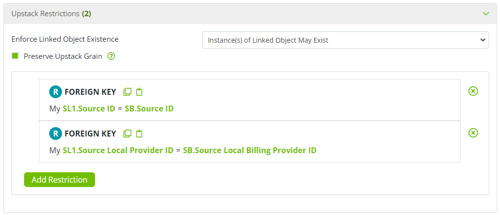
Data model keys can be generated from these crosswalk objects by linking to them using two Foreign Key patterns to join on the Source ID and the relevant "Source Local" identifier. The following screenshot shows such a link between the base object in the stack (aliased "SB") and the provider mastering object occupying the linked object 1 slot in the stack (aliased "SL1"), obtaining the mastered Provider ID value for the billing provider on a medical claim:
The mastered data model key should then be published from the Available Fields panel with the appropriate name (e.g., Billing Provider ID) and field group (i.e., Data Model Keys), as seen below.

Because patient mastering is so common, there is a dedicated pattern, Master Patient ID, that performs the equivalent logic without the need to manually link in any objects:

This pattern can be used to conveniently obtain the master Patient ID value.
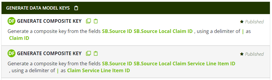
Second, for identifiers that are not mastered (typically, for example, traditional "fact table" concepts like claims, orders, labs, etc.), generating data model keys is much simpler: the Source ID value is simply prepended to the appropriate "Source Local" identifier, forming a natural key that is guaranteed to be unique in the downstream data model (assuming the source local identifier was unique in the source system). For this purpose, the Generate Composite Key pattern is a convenient substitute for the Concatenate pattern; the example below shows the generation of data model key values for Claim ID and Claim Service Line Item ID using the preferred pipe delimiter:
6. Collapsing transactional claims or billing data to final action format.
A number of previous tasks have described the data planning and preparation for reconciling transactional claims or billing data to final action format. The Local Transform layer is where the reconciliation is finally executed, by collapsing the grain of the claims table from one-record-per-transaction to one-record-per-claim or one-record-per-claim service line item.
When collapsing to final action format, the typical approach is to identify and retain only the most recent transaction in a sequence of transactions for a claim header or claim service line item. (Most often, the transactional data are at the service line item level; i.e., each transaction record modifies a distinct service line item, and different service line items on the same claim or bill can end up with different final action statuses.) Work performed in service of performing semantic mapping should already have identified the relevant fields that can be used for ordering the transactions, e.g., Transaction Sequence Number, Transaction Effective Date, etc. (See Determine the mappings for claims or billing transaction fields for a fuller description of this work.)
Recall also from this previous task that there are two prevailing conventions for storing transactional amounts:
(1) consider the values on each transaction to represent the marginal change in the amount associated with that transaction, with the final action amount obtained by summing the values across all transactions; and (2) consider the value on the last transaction to represent the final action amount.
Semantic Mapping objects should also have already labelled the relevant fields to capture the convention in use: fields like Increase to Allowed Amount and Increase to Plan Paid Amount are used for convention (1), while fields like Resulting Allowed Amount and Resulting Plan Paid Amount are used for convention (2).
With all these preparations made, the logic used in the Local Transform object is now relatively straightforward. If the data follow convention (1), use the pattern Sum Across Instances to calculate the cumulative final action amounts net of all transactions.
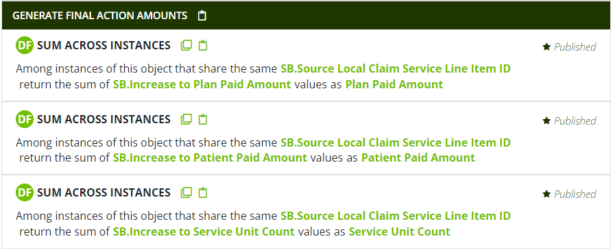
(Note, as in the example here, that some non-financial fields like Service Unit Count on medical claims and Quantity Dispensed and Days Supply on pharmacy claims may also be appropriate to include in these calculations.)
If the data follow convention (2), no special patterns are necessary to generate the final action amounts; rather, the act of excluding all but the final transaction will do the work of retaining the appropriate amounts.
Finally, to collapse to final action grain, the Keep Ordinal N pattern is typically most convenient technique:
7. Generating claim or bill header-level values based on service line items.
If working with claims or billing service line item data, after collapsing to final action status -- or if the data were already final action status -- it's often necessary to generate claim or bill header-level field values from the line-level values.
Consider the following header-level values that often need to be generated from line-level amounts:
- Aggregate header-level charged, allowed, and paid amounts
By definition, the claim or bill header-level financials should match the sum of the line-level values.
- Claim or bill reversed status
If all the service line items on a claim or bill are found to be reversed or denied as their final action status, it is generally correct to consider the entire claim or bill reversed or denied.
- Header-level covered start and end dates
The header-level covered date fields (Claim Covered Start Date and Claim Covered End Date) should, with perhaps some rare exceptions, identify the full period of services included as line items, i.e., the earliest line-level service start date to the latest line-level service end date.
Generally, all of these aggregations are accomplished in much the same way that transaction-level values were rolled up to service-line-level values. For example, the Claim Covered Start Date can be generated the Minimum Value Across Instances and Maximum Value Across Instances patterns, as shown here:
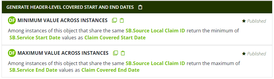
(Note that it's not necessary here to actually collapse the grain size of the data to header-level; the line-level grain can be maintained while still -- through these patterns -- generating "aggregate" field values.)
Even if the source data include some or all of these header-level values, it can be prudent to corroborate them with values obtained from an aggregation of the line-level values. To the extent these values disagree, that might be used to trigger a data integrity investigation.
8. Reshaping data from wide to long form.
It is very common for source data to represent a list of diagnosis codes in "wide form", i.e., with the different codes associated with a claim or bill or some other event as distinct columns on the same record. For example:
| Source ID | Patient ID | Claim ID | Diagnosis 1 ICD-10-CM Code | Diagnosis 2 ICD-10-CM Code | Diagnosis 3 ICD-10-CM Code | Is Diagnosis 1 Present on Admission | Is Diagnosis 2 Present on Admission | Is Diagnosis 3 Present on Admission |
|---|---|---|---|---|---|---|---|---|
| DS | MRN|1 | 10 | A01.0 | Z00.01 | B01.0 | 1 | 0 | 0 |
In contrast to this structure, the Ursa Health Core Data Model stores diagnosis codes in "long form", which plays to the strengths of relational database operations. The process of reshaping date from wide- to long-form is performed in Ursa Studio with the Reshape Wide to Long transformation pattern, shown below:
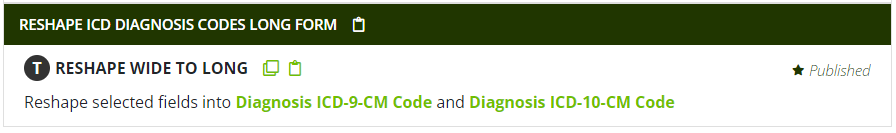
This pattern can involve multiple "banks" of fields at once; for example, if "Present on Admission" flags are included as wide-form data, both the diagnosis codes and the present on admission field values can be simultaneously reshaped. The resulting table would look like the following:
| Source ID | Patient ID | Claim ID | Diagnosis Line Number | Diagnosis ICD-10-CM Code | Is Diagnosis Present on Admission |
|---|---|---|---|---|---|
| DS | MRN|1 | 10 | 1 | A01.0 | 1 |
| DS | MRN|1 | 10 | 2 | Z00.01 | 0 |
| DS | MRN|1 | 10 | 3 | B01.0 | 0 |
9. Generating well-formed line numbers.
In the Ursa Health Core Data Model, service, procedure, and diagnosis line numbers are considered to be part of a records Data Model Key fields, and should be well-formed. For example, a convenient and performant way to collapse a collection of claim service line items to one-record-per-claim grain is to simply add a restriction pattern for Service Line Number = 1; but this sort of operation only works if there is always exactly one service line item record on a claim with Service Line Number = 1.
To be precise, a well-formed line number field starts at 1 (within some appropriate scope, e.g., a claim) and increments by 1 for each new line.
This kind of well-formed line number can be guaranteed by using the Ordinal Rank Among Instances pattern with a sort ordering based on the original source data line numbers; for example:

10. Setting validation rules.
As with all objects, Local Transform objects can be imbued with validation rules that fire every time the object is run.
The rules framework implemented in Ursa Studio is very flexible, and teams can get creative with how to use them, but a best practice is to at least use validation rules to test for violations of key assumptions that, if violated, would cause irreparable harm to logic in the current object or in downstream objects. It is especially important to catch these kinds of violations if they would otherwise fail "silently" -- i.e., without error -- leaving users unaware that their analytic results might be fatally compromised.